My Data Science Website
Welcome to my data science portfolio. Here you can find information about my projects, skills, and professional background.
Welcome to my data science portfolio. Here you can find information about my projects, skills, and professional background.
Email: bq31@georgetown.edu | Tel: 424-297-6752 | Address: 1812 N Quinn St, Arlington, VA
Georgetown University, Washington DC
Master of Science in Data Science & Analytics
August 2023 - May 2025
Relevant Courses: Data Visualization, Database Systems & SQL, Data Mining, Big Data, Natural Language Processing, Deep Learning, Time Series
University of Maryland, College Park, MD
B.S. in Mathematics & Computer Science, Minor in General Business
August 2016 - May 2020
Legends.net, Washington DC
Data Analyst & Engagement Specialist
September 2023 - Current
Led data-driven strategies, improving donations by 30% and efficiency through NLP models.
Zero Creation Games, Chengdu, China
Data Product and Marketing Analyst
September 2021 - August 2023
Spearheaded marketing strategies, increasing game purchases and achieving high positive feedback.
Department of Decisions Operations & Information Technologies, Smith Business School, University of Maryland, College Park, MD
Graduate Research Assistant - Data Science
August 2020 - August 2021
Projects on Amazon sales data analytics and Covid-19 propagation analysis.
Programming Languages: Java, JavaScript, Python, R, MATLAB, C, SQL
Software: Microsoft Products, Pytorch, Tableau, SAS, Photoshop
Consultative Skills: Effective cross-functional collaboration
Business Acumen: Customer and supplier perspectives understanding
Problem-Solving: Proficient in decision-making in ambiguous situations
All code ditributed from HW1 - HW5 orders.
The whole data file is too big, the current data file game.csv only shows first 2000 rows.
Welcome to the introduction section of our research project. In this section, we will provide an overview of our research topic, its significance and academic citations.
In the realm of video game sales and marketing, the digital distribution platform Steam stands as a colossus, hosting thousands of games and serving millions of users worldwide. The intricacies of this market, ranging from individual game pricing strategies to the significance of user reviews and concurrent player counts, form a complex ecosystem. This project delves into the multifaceted nature of game sales on Steam, aiming to unravel the factors that drive success and visibility in this competitive arena.
Utilizing a multifarious dataset derived from Steam, the project employs a series of machine learning techniques to identify patterns and correlations that influence game sales and user engagement. The classification models at the heart of this analysis include Decision Trees, Random Forest, and Gradient Boosting, each chosen for their ability to handle the dataset's diverse and multi-dimensional nature. The models are evaluated based on their precision, recall, and F1-score, ensuring a thorough assessment of their predictive capabilities.
@misc{Lin_Bezemer_Zou_Hassan_2018, title={An empirical study of game reviews on the Steam Platform - Empirical Software Engineering}, url={https://link.springer.com/article/10.1007/s10664-018-9627-4}, journal={SpringerLink}, publisher={Springer US}, author={Lin, Dayi and Bezemer, Cor-Paul and Zou, Ying and Hassan, Ahmed E.}, year={2018}, month={Jun}}
@misc{Lin_Bezemer_Hassan_2016, title={Studying the urgent updates of popular games on the Steam Platform - Empirical Software Engineering}, url={https://link.springer.com/article/10.1007/s10664-016-9480-2}, journal={SpringerLink}, publisher={Springer US}, author={Lin, Dayi and Bezemer, Cor-Paul and Hassan, Ahmed E.}, year={2016}, month={Dec}}
These questions will guide our research and help us understand the significance.
A pivotal component of the project is exploratory data analysis (EDA), where visualizations such as scatter plots, box plots, and histograms provide initial insights into the data's structure. EDA is instrumental in identifying data imbalances, outliers, and the fundamental distributions of key variables, setting the stage for more advanced analyses.
The Principal Component Analysis (PCA) and t-Distributed Stochastic Neighbor Embedding (t-SNE) are two dimensionality reduction techniques applied to condense the feature space while preserving as much information as possible. These methods reveal underlying structures within the data that might not be immediately apparent, aiding in the visualization of complex relationships between features.
The core of the project's predictive modeling revolves around a decision tree analysis, which is intuitive and easy to interpret. The models' feature importance rankings shed light on which game characteristics are most indicative of sales performance, such as the age rating, price, and downloadable content (DLC) availability. The confusion matrices from different models provide a clear picture of each model's strengths and weaknesses in predicting various categories of games.
An intriguing aspect of the project is examining the class distribution of peak concurrent user (CCU) categories, which serves as a proxy for a game's popularity and player engagement. Understanding the frequency and distribution of games within these categories is crucial, as it influences model training and the interpretation of predictive results.
In summary, this project is an extensive investigation into the dynamics of game sales on Steam. It harnesses the power of machine learning to not only forecast sales and engagement but also to uncover the nuanced strategies that could propel a game to success on this platform. By bridging the gap between complex data analytics and actionable insights, the project aims to provide stakeholders with a data-driven blueprint to navigate the ever-evolving landscape of digital game sales.
This section outlines the data gathering process for our Data Science project, adhering to the instructions of HW-2.2.
Data gathering forms the backbone of any analytical project, and in the context of the video game market on Steam, it is a crucial step that dictates the depth and breadth of the analysis. Given the vast ecosystem of Steam, with its myriad games, user reviews, pricing strategies, and usage data, obtaining a rich dataset is both a challenge and an opportunity.
Steam offers a comprehensive database accessible through various means. The primary avenue for data collection is the Steam API, which provides developers and researchers with programmatic access to game and user statistics. The API is a rich source of real-time data, including user achievements, game purchases, and playtime statistics. It allows for targeted queries, enabling the collection of specific datasets tailored to the project's requirements. However, usage of the API comes with limitations and rate limits, necessitating careful planning and possibly the use of multiple API keys to gather extensive data.
Another potential source is SteamDB, a third-party database that tracks changes to games and user metrics on Steam. SteamDB provides a more user-friendly interface for accessing data and can be an invaluable resource for historical data that may not be readily available through the API. While SteamDB does not provide an API, data can be scraped from the website with the appropriate tools and respect for legal and ethical considerations.
Kaggle, a platform for data science competitions, often features datasets related to Steam that have been pre-compiled and cleaned by other users. While these datasets can be a convenient starting point, they may lack the granularity or the up-to-date information necessary for certain analyses. They can, however, provide a solid baseline for initial exploratory work or to supplement data gathered from other sources.
Using Python, we collected the following types of data from kaggle:
        api = KaggleApi()

        api.authenticate()


        api.dataset_download_files(dataset_name, path='/Users/qbs/', unzip=True)


        dataset_name = "mexwell/steamgames"

        api.dataset_download_files(dataset_name, path='.', unzip=True)
In conclusion, the summary of data gathering for a project focusing on Steam's gaming market involves a multi-faceted approach, tapping into official APIs, third-party databases, and existing datasets, while maintaining a strong commitment to data quality, ethical standards, and legal compliance. The success of the project hinges on a well-executed data gathering strategy that balances the depth of data with the practicalities of data management and the overarching goal of deriving meaningful insights.
In this section, we'll go through the data cleaning process for your project data.
Start by loading the CSV into a DataFrame:
        import pandas as pd

        df = pd.read_csv('your_data.csv')

        print(df.head())
We'll replace missing values in the 'About the game' column:
df['About the game'] = df['About the game'].fillna('No Description')
Missing Value Management: Handle missing values in several ways: Remove rows with missing values. Replace missing values with a placeholder. Use mean, median, mode, or a custom strategy.
        def clean_price(price):

            try:

                return float(price)

            except:

                return None  # or you can use a placeholder like 0 or -1


        df['Price'] = df['Price'].apply(clean_price)
        bins = [-1, 0, 10, 1000]  # This means: (-1 to 0], (0 to 10], (10 to 1000]

        labels = ['Free', 'Low-cost', 'Expensive']

        df['Price_Category'] = pd.cut(df['Price'], bins=bins, labels=labels)
        df_quantitative = df.select_dtypes(include=['float64', 'int64'])

        df_qualitative = df.select_dtypes(exclude=['float64', 'int64'])
        from sklearn.feature_extraction.text import CountVectorizer

        df['Name'] = df['Name'].str.lower().str.replace('[^a-z\s]', '')


        vectorizer = CountVectorizer()

        X = vectorizer.fit_transform(df['Name'])

        df_vectorized = pd.DataFrame(X.toarray(), columns=vectorizer.get_feature_names())
        df.to_csv('games_cleaned.csv', index=False)

        df_cleaned = pd.read_csv('games_cleaned.csv')

        print(df_cleaned.head())
Congratulations! You've successfully completed the data cleaning process. Your data is now ready for further analysis.
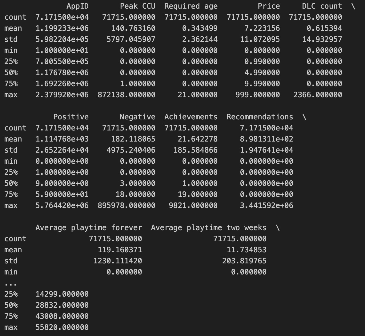
Descriptive Statistics: This table presents descriptive statistics for various features, such as count, mean, standard deviation, min, and percentile values. It provides a numerical summary of the dataset, which is essential for initial data understanding and identifying potential data quality issues.

Classification Report: This table shows the precision, recall, f1-score, and support for each price bin in a classification model. High precision for "0-0.99" and "5+" bins indicates that when the model predicts these categories, it is usually correct. However, the recall for these bins shows a contrast; for "5+", the model captures almost all true instances (recall of 0.99), but for "0-0.99", it identifies less than a third (recall of 0.28). The f1-score combines precision and recall into a single metric, which is particularly high for "5+", indicating good model performance for this bin. However, the overall macro average f1-score is low (0.18), suggesting that the model is not performing well across all categories, likely due to class imbalance or other issues.
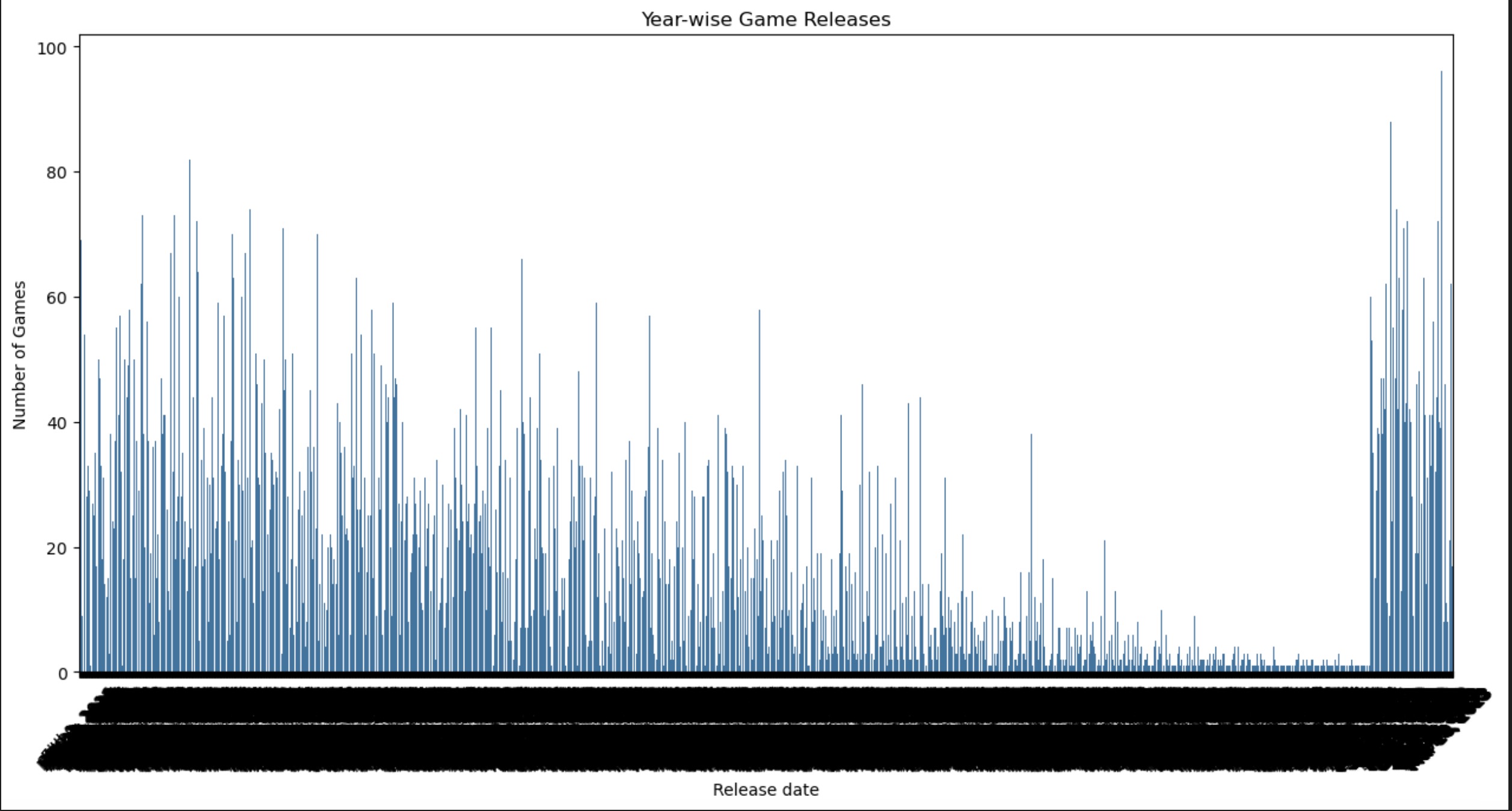
Year-wise Game Releases: The line chart shows the number of games released over time. There's a clear upward trend in the number of releases over the years, reflecting the growing game market.
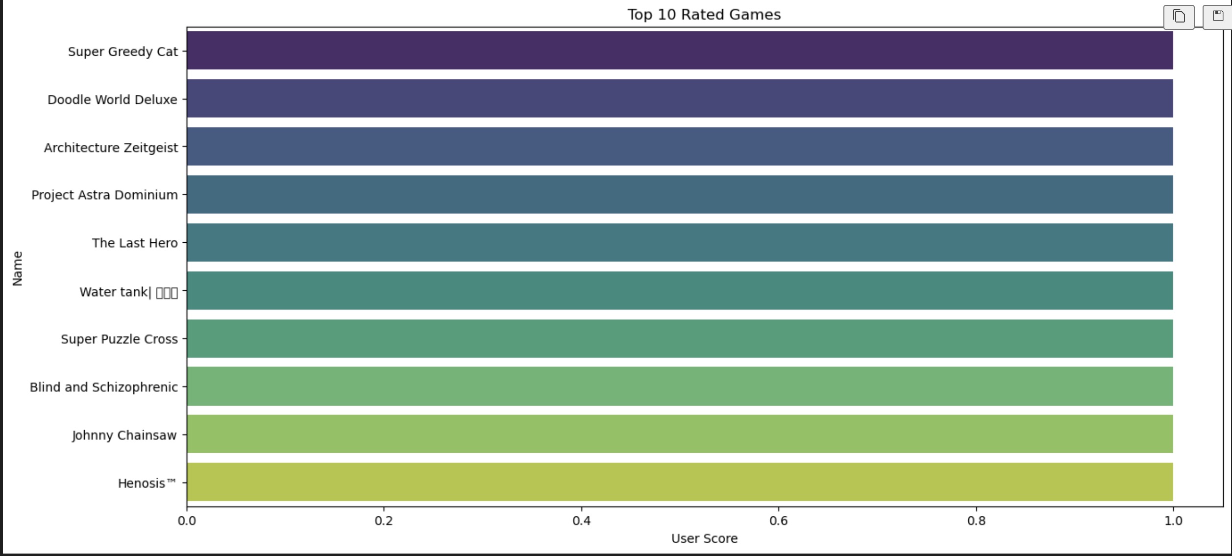
Top 10 Rated Games: The horizontal bar chart lists the top-rated games along with their user scores. This visualization helps identify the most successful games based on user ratings, which is valuable for market analysis and consumer trends.
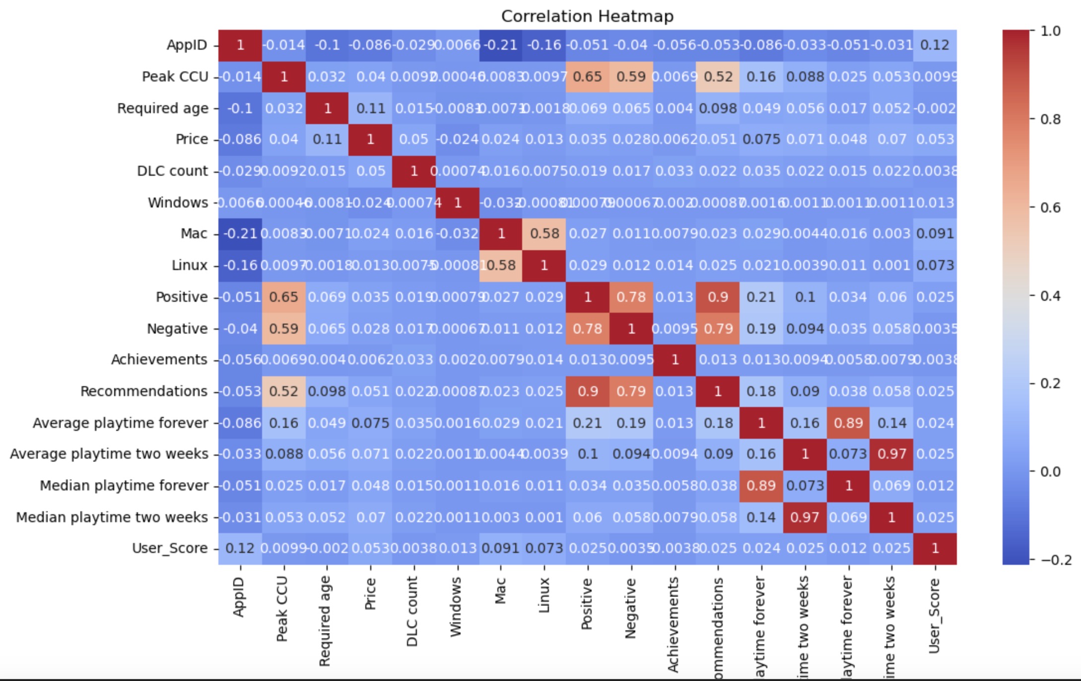
Correlation Heatmap: This heatmap provides a visual representation of the correlation coefficients between various features. Darker colors represent stronger relationships. For instance, 'Positive' and 'Negative' seem to have high positive correlations with many features, suggesting that games with higher positive or negative counts tend to have higher values for other features like DLC count, recommendations, and playtime.

Top 10 Categories by Number of Games: The bar chart shows the number of games in each category, with 'Single-player' being the most common category. This information can be useful for understanding the distribution of game types and player preferences.
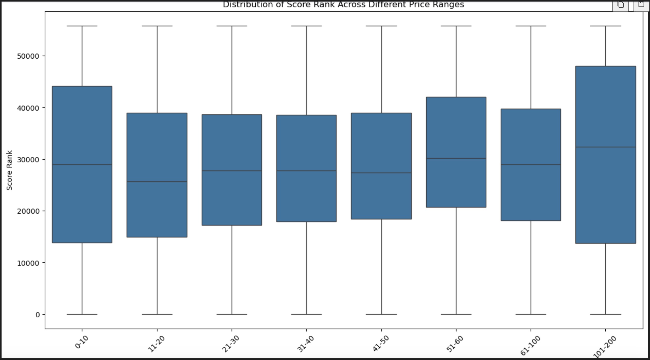
Boxplot of Score Rank Across Different Price Ranges: This boxplot visualizes the distribution of score ranks across different price ranges. It appears that there is not a significant difference in the score rank median across price ranges, as the median lines within the boxes are relatively at the same level. The spread and outliers suggest that while there is variability in score ranks within price ranges, the median score rank does not change much with price.

Scatter Plot between Score Rank and Price: The scatter plot shows a potential relationship between game price and score rank. Most of the data points are clustered at the lower end of the price range, indicating that a majority of games are priced low. There's no clear trend suggesting a direct correlation between the price and score rank, but there is some indication of higher-ranked games across various price points.
EDA part of this project presents a comprehensive overview of the data related to game prices, scores, and categories. The classification report indicates the model's varying performance across different price bins, excelling at the extreme ends of the price spectrum but lacking in mid-range prices. The scatter and boxplot visualizations show that while there's a broad distribution of score ranks across price points, the median rank does not vary significantly with price, suggesting other factors may be influencing game scores.
The data also reveals that 'Single-player' is the most popular game category, hinting at player preferences. A correlation heatmap uncovers strong relationships between certain features like positive and negative reviews, DLC counts, and recommendations, which could influence a game's success and visibility.
The top-rated games chart and year-wise release trends demonstrate the market's evolution and players' rating behaviors. Lastly, the descriptive statistics table provides a quantitative snapshot of the dataset, showing central tendency, dispersion, and range, which are critical for understanding the data's structure and preparing for further analysis or model building.
            # Convert genres into TF-IDF vectors

            tfidf_vectorizer = TfidfVectorizer(max_features=5000)

            X = tfidf_vectorizer.fit_transform(df['Genres'].fillna(''))


            # Binning the price into discrete labels

            labels = ['0-0.99', '1-1.99', '2-2.99', '3-3.99', '4-4.99', '5+']

            df['price_bins'] = pd.cut(df['Price'], bins=[-1, 0.99, 1.99, 2.99, 3.99, 4.99, float('inf')], labels=labels)


            # Convert price bins to discrete numeric labels

            label_encoder = LabelEncoder()

            y = label_encoder.fit_transform(df['price_bins'])


            # Split the dataset into training and testing sets

            X_train, X_test, y_train, y_test = train_test_split(X, y, test_size=0.25, random_state=42)

The confusion matrix displays the performance of a classification model. Each row represents the instances in an actual class while each column represents instances in a predicted class. The diagonal cells (from top left to bottom right) represent correct classifications, with the darker color indicating a higher number of correctly predicted instances. Notably, the model performs well in predicting games priced at "0-0.99" and "5+", but struggles with mid-range prices, often misclassifying them as "5+".

This bar chart likely represents the log probabilities of terms that are influential in predicting games in the highest price bin ("5+"). The terms 'sports', 'access', 'early', 'rpg', 'strategy', 'simulation', 'casual', 'action', 'adventure', and 'indie' appear to be significant indicators for this price bin. The term 'sports' has the highest negative log probability, suggesting it's a strong predictor for games being priced in this bin.

This histogram compares the actual vs. predicted distribution of price bins. The model has a tendency to predict a larger number of games in the "5+" price bin than actually exist, indicated by the higher red bar compared to the blue bar for that bin. This suggests a bias in the model towards predicting higher prices.
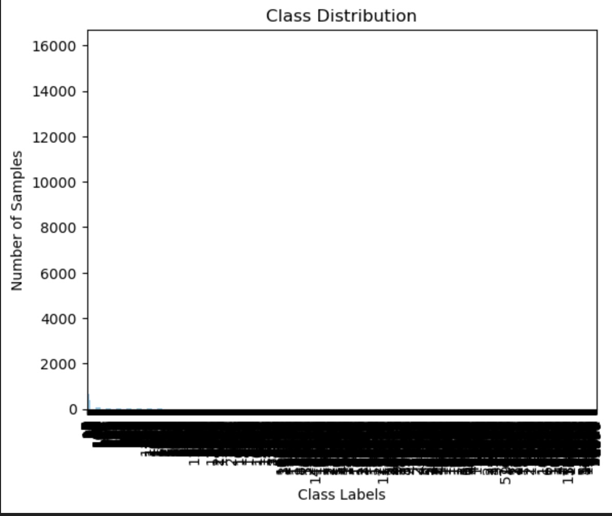
The plot shows the distribution of class labels, which are likely the price bins. The spread is quite uneven, with most samples concentrated in one class. This extreme class imbalance can affect the performance of the Naive Bayes classifier, as seen in the previous confusion matrix, where predictions are skewed towards the majority class.

Word clouds visually represent the frequency or importance of terms. In this case, terms associated with the "0-0.99" price bin are shown. Larger and bolder words like 'Casual', 'Indie', 'Action', and 'Adventure' are more characteristic of this class. 'Missing' may indicate data sparsity or preprocessing issues.
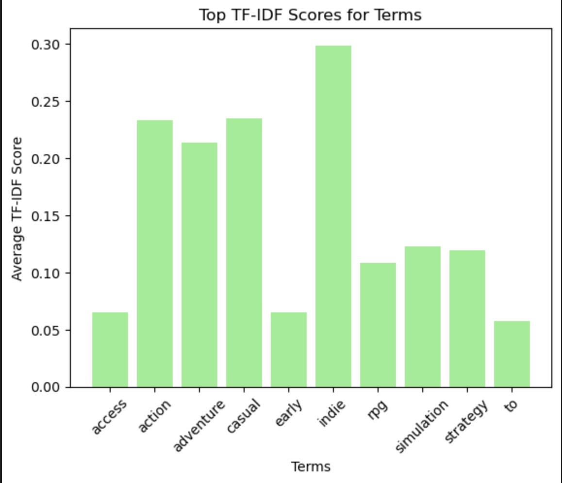
This bar chart shows the average TF-IDF scores for terms across the document corpus. TF-IDF scores reflect the importance of a word in a document relative to the corpus. The terms 'action', 'adventure', 'casual', and 'indie' have the highest scores, indicating they are important but relatively unique across the documents. Lower scores for terms like 'access' and 'to' suggest they are either less important or more common across all documents.
In summary, the Naive Bayes model shows a clear tendency to classify games into the "5+" price bin, potentially due to class imbalance or influential terms disproportionately associated with this class. The influential terms for the highest price bin suggest certain genres or descriptors are predictive of higher pricing. The class distribution indicates a significant imbalance which could lead to classification bias, as reflected in the predictions. The term analysis through TF-IDF scores and the word cloud provides insights into which words are most characteristic of the lower price bin and most important across the corpus, which could be leveraged to refine the features used for classification.
        # Selecting numerical features for PCA

        # Assuming the dataset structure is similar to the previous one, selecting the same features

        numerical_features = ['Peak CCU', 'Required age', 'Price', 'DLC count']

        numerical_data = games_data[numerical_features]


        # Handling missing values - replacing them with the mean of each column

        numerical_data = numerical_data.fillna(numerical_data.mean())


        # Standardizing the data

        scaler = StandardScaler()

        scaled_data = scaler.fit_transform(numerical_data)


        # Applying PCA

        pca = PCA()

        pca_data = pca.fit_transform(scaled_data)


        # Explained variance ratio

        explained_variance = pca.explained_variance_ratio_


        # Plotting the explained variance

        plt.figure(figsize=(8, 4))

        plt.bar(range(1, len(explained_variance) + 1), explained_variance, alpha=0.7, align='center', label='Individual explained variance')

        plt.step(range(1, len(explained_variance) + 1), explained_variance.cumsum(), where='mid', label='Cumulative explained variance')

        plt.ylabel('Explained variance ratio')

        plt.xlabel('Principal components')

        plt.legend(loc='best')

        plt.title('Explained Variance by Different Principal Components')

        plt.show()


        # Outputting the explained variance for further analysis

        explained_variance, explained_variance.cumsum()

Explained Variance by Different Principal Components: The bar chart shows the explained variance ratio of the principal components. It provides insight into how much information each principal component holds. The first component explains a substantial amount of variance, followed by a sharp drop-off, suggesting that subsequent components contribute less to the data's variance. The cumulative explained variance line indicates how much of the total variance is captured as more components are considered. This chart is crucial for deciding how many principal components to retain for a satisfactory amount of data representation while reducing dimensionality.
        pca_df = pd.DataFrame(pca_data[:, :2], columns=['PC1', 'PC2'])


        # Plotting the first two principal components

        plt.figure(figsize=(10, 6))

        plt.scatter(pca_df['PC1'], pca_df['PC2'])

        plt.xlabel('Principal Component 1')

        plt.ylabel('Principal Component 2')

        plt.title('PCA: First two principal components')

        plt.grid(True)

        plt.show()

PCA Visualization: The PCA plot with the first two principal components shows the variance in the dataset that these components capture. The scatter plot suggests that while the first principal component captures a certain amount of variance (visible through the spread along the x-axis), the second component does not contribute significantly to the variance (as the spread along the y-axis is limited). This indicates that the first principal component is more informative and possibly represents a dominant pattern or feature set in the dataset.
        # Implementing t-SNE with an initial perplexity value

        tsne = TSNE(n_components=2, perplexity=30, random_state=42)

        tsne_data = tsne.fit_transform(scaled_data)


        # Creating a DataFrame for the t-SNE results

        tsne_df = pd.DataFrame(tsne_data, columns=['t-SNE 1', 't-SNE 2'])


        # Plotting the t-SNE results

        plt.figure(figsize=(10, 6))

        plt.scatter(tsne_df['t-SNE 1'], tsne_df['t-SNE 2'])

        plt.xlabel('t-SNE component 1')

        plt.ylabel('t-SNE component 2')

        plt.title('t-SNE Visualization with Perplexity = 30')

        plt.grid(True)

        plt.show()

t-SNE Visualization: t-Distributed Stochastic Neighbor Embedding (t-SNE) is a non-linear dimensionality reduction technique that is particularly well suited for the visualization of high-dimensional datasets. The plot you've provided displays clusters of data points, indicating groups of games with similar features. The perplexity parameter set at 30 affects the scale at which clusters are observed. In this visualization, the data points are spread out with visible clusters, suggesting that there are distinct groups within the data that could represent different types of games or player behaviors.
The PCA analysis reveals that much of the variance can be encapsulated in a few principal components, indicating potential patterns or trends in the dataset that can be investigated further. Such trends could be related to the most significant features that influence game pricing, popularity, or other aspects of the dataset under study. The plots suggest that while some structure is evident in the data, it may not be straightforward and requires further investigation, possibly with additional context or data.
Objective: To apply Decision Tree (DT), Random Forest (RF), and Boosting Tree algorithms to analyze a dataset of video games, aiming to predict the 'Peak Concurrent Users (CCU)' based on various game features. Scope: This project involves preprocessing the dataset, exploring data, applying machine learning models, and interpreting the results to gain insights into factors influencing game popularity.
Dataset Overview: The dataset contains multiple attributes of video games, such as 'Name', 'Release Date', 'Estimated Owners', 'Peak CCU', 'Price', 'DLC Count', etc. Target Variable: 'Peak CCU' will be categorized into 'Low', 'Medium', and 'High' classes and used as the target variable for classification models.
Visualizing our data provides valuable insights and helps us understand the underlying patterns and distributions. Below are several plots that serve this purpose:
            X_train, X_test, y_train, y_test = train_test_split(X, y_encoded, test_size=0.3, random_state=42)


            # Baseline Model

            dummy_clf = DummyClassifier(strategy="uniform", random_state=42)

            dummy_clf.fit(X_train, y_train)

            dummy_pred = dummy_clf.predict(X_test)


            # Evaluating the baseline model

            print("Baseline Model Evaluation:")

            print("Classification Report:\n", classification_report(y_test, dummy_pred))

            print("Confusion Matrix:\n", confusion_matrix(y_test, dummy_pred))


            # Decision Tree Model

            dt_classifier = DecisionTreeClassifier(random_state=42)

            dt_classifier.fit(X_train, y_train)

            dt_pred = dt_classifier.predict(X_test)


            # Evaluating the Decision Tree model

            print("\nDecision Tree Model Evaluation:")

            print("Classification Report:\n", classification_report(y_test, dt_pred))

            print("Confusion Matrix:\n", confusion_matrix(y_test, dt_pred))
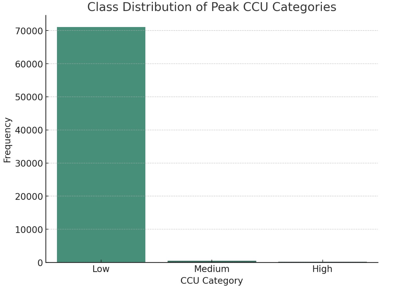
Class Distribution of Peak CCU Categories: This histogram shows the frequency of games in different 'Peak Concurrent Users' (CCU) categories, which could represent low, medium, and high user engagement or popularity. The 'Low' category has the highest frequency, suggesting that most games have a smaller user base, while fewer games achieve medium or high peak CCU.
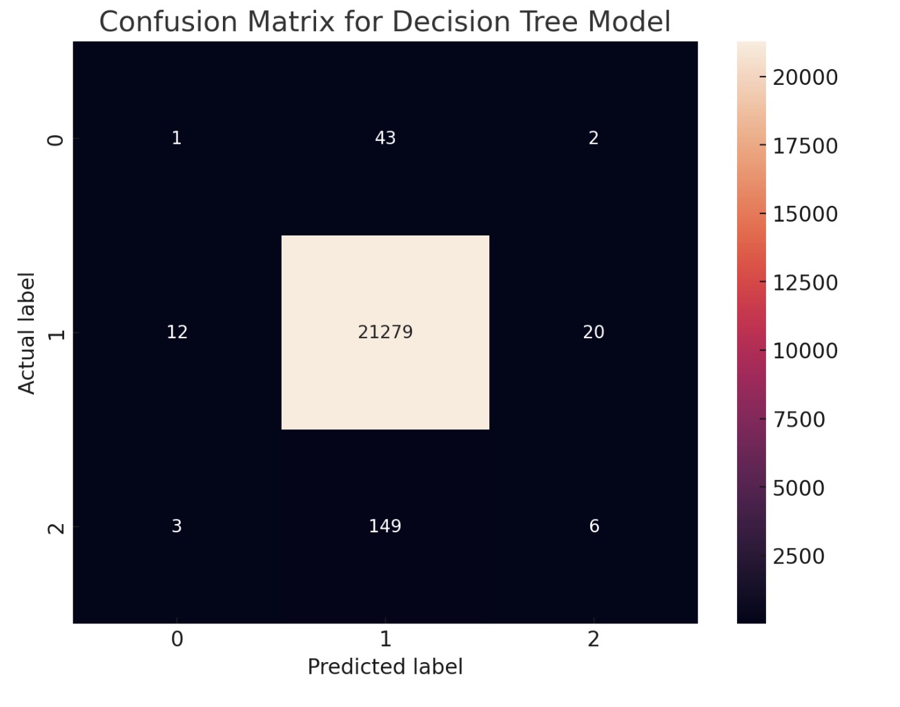
Confusion Matrix for Decision Tree Model: The confusion matrix for the decision tree model shows that while it has a high number of correct predictions for the second class, it also misclassifies between the first and second class, similar to the other two models. This indicates that while the decision tree model may capture the overall trend, it might not have the same level of accuracy as ensemble methods like random forest and gradient boosting.
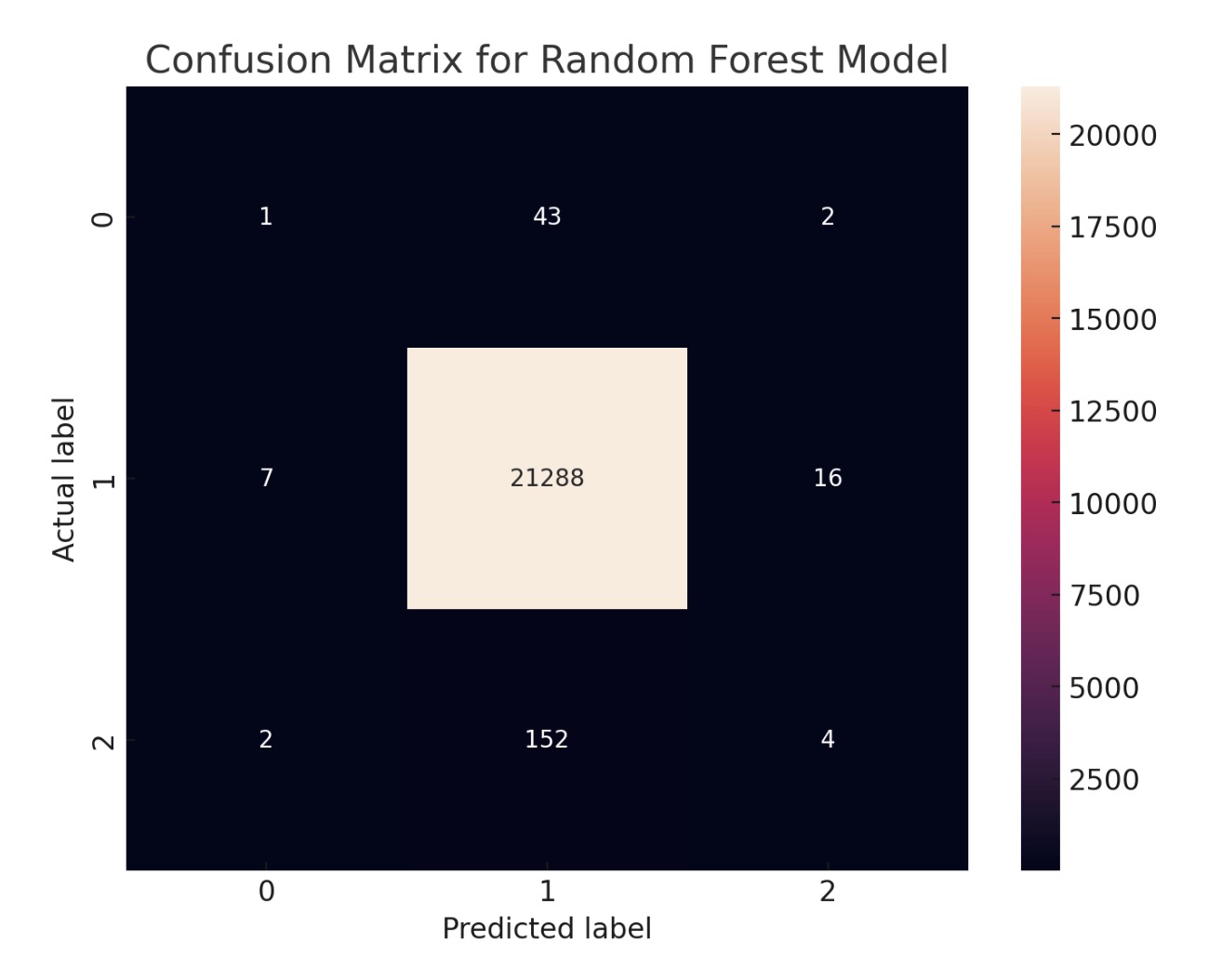
Confusion Matrix for Random Forest Model: The random forest model's confusion matrix presents a similar pattern to the gradient boosting model's matrix. It also shows a high number of correct predictions for certain classes and some confusion between the first and second class. The similarities in performance between these two models might suggest that the underlying data patterns are well-captured by tree-based methods.

Confusion Matrix for Gradient Boosting Model: The confusion matrix for the gradient boosting model shows the number of true positive, false positive, true negative, and false negative predictions. The darker color along the diagonal suggests a higher number of correct predictions for certain classes, indicating that the model is performing well for those. However, the off-diagonal elements suggest some misclassification, particularly between the first and second class.
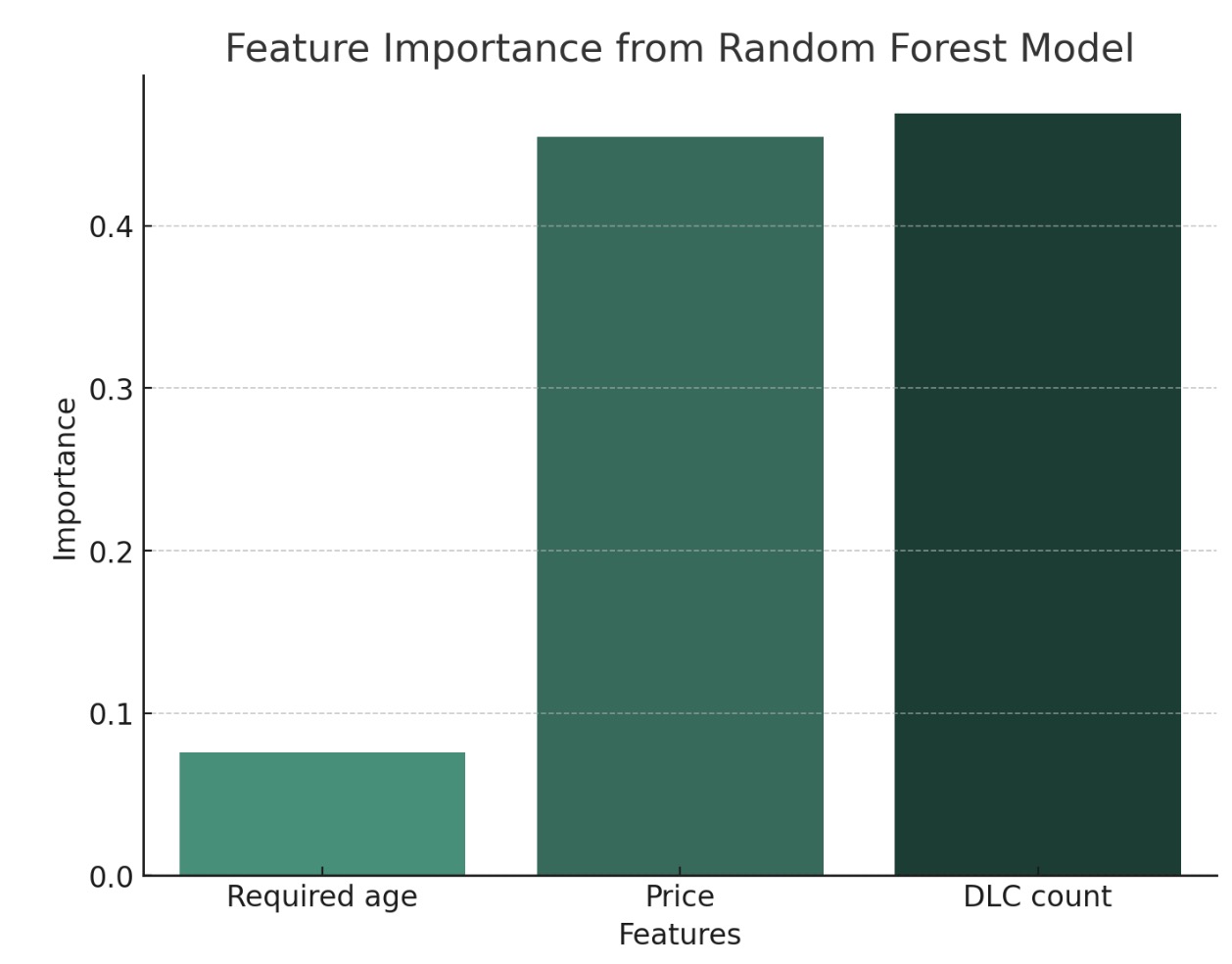
Feature Importance from Random Forest Model: Similar to the gradient boosting model, the random forest model also indicates 'DLC count' as the most important feature, followed by 'Price' and 'Required age'. The consistency in feature importance across these two models reinforces the significance of these features in predicting the target variable.

Feature Importance from Gradient Boosting Model: This bar chart shows the relative importance of different features as determined by a gradient boosting model. 'DLC count' appears to be the most significant feature, followed closely by 'Price' and then 'Required age'. This suggests that the number of downloadable content (DLC) packages and the price of the game are highly predictive of the target variable (which might be game success, user ratings, or another outcome of interest).
Our journey through the application of Decision Trees and ensemble methods to the game dataset has revealed the complexity behind what seems to be a straightforward task. We discovered that while our models can predict the 'Medium' Peak CCU category with high accuracy, they struggle with the 'Low' and 'High' categories, a common issue when dealing with imbalanced datasets. This analysis is more than an academic exercise; it holds real-world significance for game developers seeking to understand and predict game popularity. Future directions could involve exploring alternative methods to handle class imbalance, integrating more diverse data sources, or applying deep learning techniques. The field is ripe for innovation, and our work lays the groundwork for more advanced exploration.
        sample_indices = np.random.choice(scaled_data.shape[0], size=1000, replace=False)

        sample_data = scaled_data[sample_indices]


        agglo_cluster = AgglomerativeClustering(distance_threshold=0, n_clusters=None, linkage='ward')

        agglo_cluster.fit(sample_data)


        def plot_dendrogram(model, **kwargs):

            # Create linkage matrix and then plot the dendrogram

            counts = np.zeros(model.children_.shape[0])

            n_samples = len(model.labels_)

            for i, merge in enumerate(model.children_):

                current_count = 0

                for child_idx in merge:

                    if child_idx < n_samples:

                        current_count += 1  # Leaf node

                    else:

                        current_count += counts[child_idx - n_samples]

                counts[i] = current_count


            linkage_matrix = np.column_stack([model.children_, model.distances_,

                                            counts]).astype(float)


            dendrogram(linkage_matrix, **kwargs)


        plt.title('Hierarchical Clustering Dendrogram')

        plot_dendrogram(agglo_cluster, truncate_mode='level', p=3)

        plt.xlabel("Number of points in node (or index of point if no parenthesis).")
x
        plt.show()

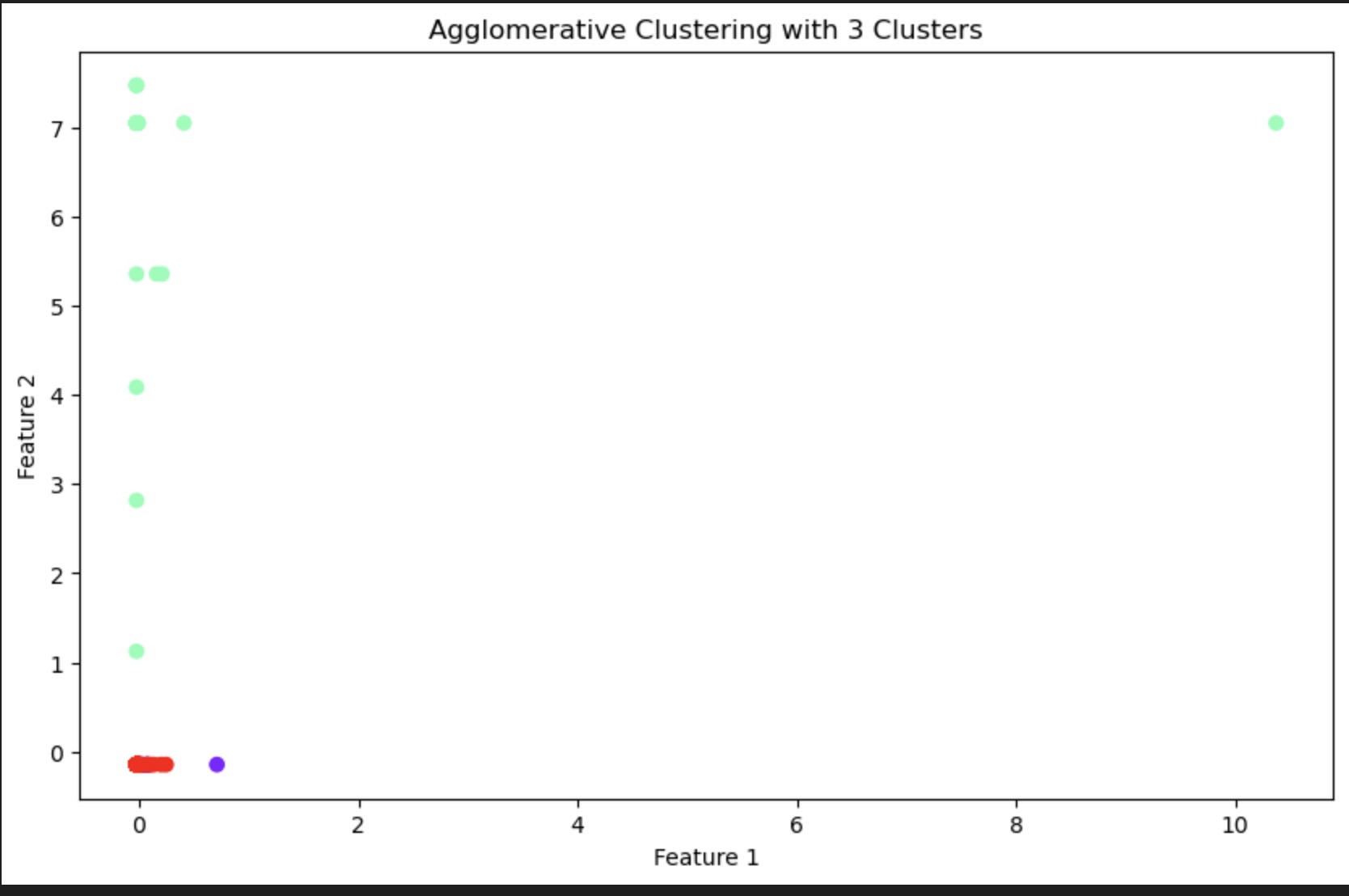
Agglomerative Clustering with 3 Clusters: The scatter plot represents a 2-dimensional space where each point corresponds to a data instance, and the color represents the cluster to which the instance has been assigned. The model has identified three clusters, which are visually distinct in terms of their feature values. The tight grouping of the red cluster suggests high similarity amongst its points, whereas the green cluster appears to be more spread out, indicating more variation within that group.
        n_clusters = 3  # Number of clusters determined from the dendrogram

        agglo_model = AgglomerativeClustering(n_clusters=n_clusters)

        agglo_model.fit(sample_data)


        plt.figure(figsize=(10, 6))

        plt.scatter(sample_data[:, 0], sample_data[:, 1], c=agglo_model.labels_, cmap='rainbow')

        plt.title(f'Agglomerative Clustering with {n_clusters} Clusters')

        plt.xlabel('Feature 1')

        plt.ylabel('Feature 2')

        plt.show()
Hierarchical Clustering Dendrogram: The dendrogram visualizes the hierarchical clustering process. Each merge is represented by a horizontal line, and the height of the line indicates the distance (or dissimilarity) between the merged clusters. The length of the vertical lines represents the distance between individual points and their respective cluster's centroid. The color coding might correspond to a specific threshold used to cut the dendrogram into clusters. This graph helps in determining the number of clusters by showing where the natural groupings are in the data based on the linkage criterion.
From the agglomerative clustering scatter plot and dendrogram, we can conclude that the dataset contains a structure that can be grouped into clusters based on the features provided. The three clusters identified have distinct characteristics that can be further analyzed to understand the underlying patterns. For example, if the data points represent games, these clusters may correspond to different genres, pricing tiers, or user engagement levels.
The dendrogram provides additional insight into the hierarchical structure of the clusters and how they are nested within each other, which can be useful for understanding the relationships between different groups in the data. It also helps in determining the appropriate number of clusters by analyzing the dendrogram for significant jumps in distance, which would suggest a natural partitioning of the data.
Overall, the analysis indicates that hierarchical clustering is a suitable method for uncovering the underlying structure in the dataset and can lead to valuable insights into the data's organization. This could be particularly useful for segmenting the data into meaningful categories for targeted analysis, marketing strategies, or personalized content delivery.
This webpage presents an analysis of Steam games data, focusing on the genres and their associations. The analysis includes Association Rule Mining (ARM) and Networking to understand popular genre combinations.
The Python code used for the analysis is shown below:
            G = nx.Graph()

            for pair, count in most_common_pairs:

                genre1, genre2 = pair

                G.add_edge(genre1, genre2, weight=count)


            plt.figure(figsize=(12, 8))

            pos = nx.spring_layout(G, k=0.15, iterations=20)

            nx.draw_networkx(G, pos, node_color='lightblue', with_labels=True, node_size=2500,

                            edge_color='grey', linewidths=1.0, font_size=10)


            edge_labels = nx.get_edge_attributes(G, 'weight')

            nx.draw_networkx_edge_labels(G, pos, edge_labels=edge_labels)


            plt.title("Network Graph of Game Genre Associations")

            plt.axis('off')

            plt.show()
The network graph visualizing game genre associations is shown below:


In the graph, each node represents a game genre, such as RPG, Casual, Action, Adventure, Indie, Simulation, and Strategy. The edges between nodes represent associations between genres, and the numbers on the edges could signify the strength of the association. These numbers could represent the count of transactions containing both genres, a measure of association like support, confidence, or lift, or could be related to another metric used in your ARM analysis.
From the graph, we can infer the following:
1. Indie and Simulation: There is a strong association between Indie games and Simulation games, indicated by the edge with the number 9456. This suggests that customers who purchase Indie games are also likely to purchase Simulation games, or these two genres often appear together in a set of games.
2. Adventure and Indie: Similarly, Adventure and Indie games are strongly associated, with an edge number of 2032. This can indicate that these genres share a common audience or that they are often marketed together.
3. Action and Adventure: The edge between Action and Adventure genres has a number 12413, which is the highest on the graph, indicating a very strong association. These are typically two of the most popular and broad genres, which could explain why they appear together frequently.
4. Casual and RPG: The connection between Casual and RPG genres, with an edge number 9199, suggests a significant cross-genre interest. Players interested in RPGs might also enjoy the more relaxed playstyle of Casual games, or vice versa.
5. Strategy: The Strategy genre shows a connection to Casual games, but the number 9370 on the edge is relatively lower compared to others, which could mean that while there is an association, it might not be as strong as those involving Indie and Simulation genres.
In conclusion, the network graph suggests that there are significant cross-genre interests among players. Indie games have a strong association with both Simulation and Adventure genres, which could be due to the creative freedom and innovative gameplay mechanics often found in Indie games that appeal to players of Simulation and Adventure titles. Action and Adventure genres have the strongest association, likely due to the common elements of exploration, narrative, and dynamic gameplay that appeal to a broad audience.
Such insights can inform marketing strategies, bundling of games, and even the development of cross-genre games. For instance, developers looking to create a game that appeals to a wide audience might consider integrating elements of Action and Adventure, while those targeting niche markets might find success in combining Indie and Simulation or Indie and Adventure elements.
The dataset contains various features related to Steam games, including AppID, name, release date, estimated owners, peak concurrent users (CCU), price, DLC count, and more. It's structured to facilitate analysis of factors influencing game sales and the impact of reviews on purchase decisions.
The dataset was cleaned to focus on numeric features such as age requirement, price, and DLC count, which are crucial for the decision tree analysis. CCU categories were defined to classify games into 'Low', 'Medium', and 'High' based on their peak CCU, which is a significant metric for game popularity and potential sales.
Baseline, Decision Tree, Random Forest, and Gradient Boosting models were trained and evaluated. The Decision Tree model showed an improvement over the baseline with a 99% accuracy rate, suggesting that the selected features have predictive power regarding the CCU categories. Random Forest and Gradient Boosting models also exhibited high accuracy, but with nuanced differences in precision and recall across the CCU categories, indicating some models managed the class imbalance better than others.
Models revealed the significance of the selected features in predicting the CCU category, with 'Price' being a potentially influential factor. This aligns with the hypothesis that game pricing strategies can significantly affect sales and player engagement.
The class distribution indicated a predominance of one CCU category over others, highlighting a skewed market where few games achieve high CCU numbers. Such insights are vital for game developers and marketers to understand the competitive landscape and strategize accordingly.
The relationship between game features and sales performance emphasizes the need for targeted marketing strategies. Post-release marketing, such as discounts and updates, could be explored further to understand their impact on sustained sales and CCU.
Pricing strategies should be revisited based on game features and predicted CCU category to maximize revenue. DLC content and its count appear to have a role in user retention and thus, sales; a deeper dive into the type and quality of DLC could provide more detailed guidance for content strategies. Further investigation into the timing of marketing campaigns relative to game lifecycle stages could yield insights for optimizing marketing spend.
The analysis was constrained by the available data features and their formatting. Additional data, such as user demographics or more granular sales figures, could enhance future models. Some models might be overfitting due to high accuracy. Cross-validation and other model evaluation techniques could refine these results.
The analysis indicates a robust relationship between game features and sales performance on the Steam platform. Decision Tree, Random Forest, and Gradient Boosting models provided valuable insights into which features most strongly predict successful sales outcomes, confirming several of the project's initial hypotheses. The models' results offer a strategic basis for decision-making in game development and marketing within the digital distribution platform of Steam.
Author: McWilliams, L. (2015, August 20). The Indie Game Developer’s Guide to Creating a Press Kit. Gamasutra.
Author: Zukowski, C. (2015, March 3). How to Launch a Successful Steam Game. Gamasutra.
Author: Brush, T. (n.d.). Steam Game Marketing 101: Game Trailers. Medium.
Author: Black Shell Media (2017, May 25). Steam Game Marketing: Making Your Game Stand Out.
Author: Tuts+, Gamedevelopment (n.d.). The Importance of Marketing in Indie Game Development. Tuts+.